If you have any interest in using quantum computers today, you might have considered what it takes to simulate one (on a laptop or desktop), since fault-tolerant quantum computers are currently a rare and expensive commodity, to say the least. “Simulation” of a quantum computer might include modeling noise and pulse-level control processes, in order to better understand prototype quantum computer hardware; “emulation” is anything that gets us closer to providing the utility of a quantum computer, without a quantum computer, with rather just a desktop, laptop, or even mobile (or any other) “classical” computer device on hand.

Many experts divide the existing set of “well-known” quantum computer simulation and emulation techniques into “Schrödinger picture” and “tensor networks” (descending in part from von Neumann’s density matrices). As for what typifies “Schrödinger picture,” it basically boils down to state vector simulation (according to many others). The truth is, state vector simulation is a very simple algorithm that relies on “Schrödinger picture” interpretation or approach to quantum theory, but it is far from exhausting the extent of possible useful algorithms in the category.

Say that I ask you to simulate a circuit that produces state |control> from |0>; you do this by any means you deem fit and give me state |experiment> as output; I check that |<control|experiment>|²=1`. Why does this specifically have to occur via only state vector simulation or (von Neumann’s) tensor networks? It doesn’t.

By the way, we could even relax the |<control|experiment>|²=1 condition. (That is “Schrödinger picture,” to grant a fair point.) In cases, we could relax the condition to say, “Simulation (or emulation) provides a reusable function that accurately generates measurement shots (without bias) from the distribution of measurement in some arbitrary but user-selected basis, from a circuit definition that should produce |control> (according to my full knowledge of |control> and that |<control|experiment>|²=1, following the Born rules).”

While they are also “Schrödinger picture” (if we are limited in their modification and adaptation to our own purposes), at least “quantum binary decision diagrams” (QBDD) and “(near-)Clifford” families of simulation algorithms also exist, which can represent and compute on restricted or universal state spaces within a qubit Hilbert space. There are also other potential optimization approaches on Schrödinger picture that could constitute meaningful topics of study in themselves, I say as lead author of the Qrack simulation framework.

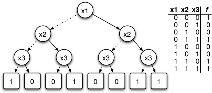
“Quantum binary decision diagrams” (QBDD) consider the quantum state to be the (multiplicative) product of “n” successive (superposed) decisions between |0> and |1> for n qubits. Each |0> and |1> possibility carries its own complex scale factor. It is possible to demand that each and every branch pair of |0> and |1> decision possibilites that share the same immediate parent node all locally normalize to 1.0 or 100% overall probability between these two options within each binary decision (but some additional complexity savings might be possible by relaxing this hypothetical condition and “telescoping” multiple levels of decision scale factors in local regions of the tree). The amplitude of a state {|0>, |1>}^⊗n is given by the product of |0> or |1> scale factor at each and every level of the tree. If a scale factor is 0, we terminate the branch at that point (compressing the tree). If two subtrees are the same, we replace their root branches with a “pointer” to the same subtree, reusing memory (and compressing the tree). Additionally, there is a global normalization condition, that the |0>-most branch with nonzero scale always carries phase angle 0 (up to non-observable global phase offset).

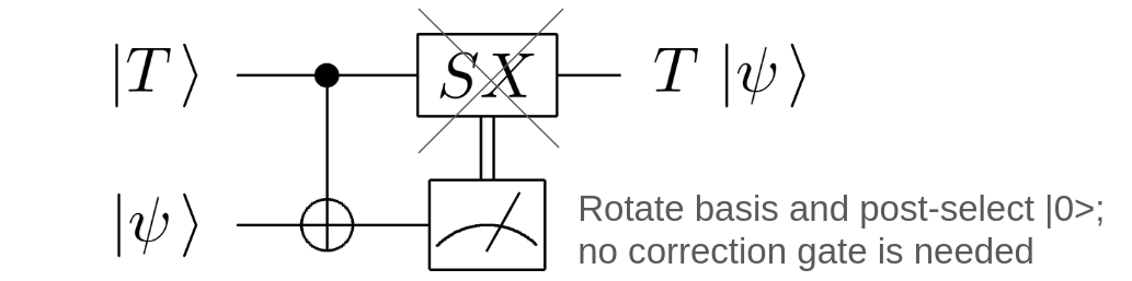
“Near-Clifford” simulation expands stabilizer simulation to encompass universal quantum computation. As you might know, according to Gottesman-Knill theorem, stabilizer tableau (as per Scott Aaronson’s CHP simulator) is efficient for Clifford algebra, which can represent superposition and entanglement but not general universal quantum states or computation. However, as near-Clifford simulation is done (rather uniquely) in the Qrack simulator framework, “magic” gates like T or RZ can be injected via “gadgets.” If a gadget ancilla is rotated to a specific basis and post-selected for |0> measurement outcome, no semi-classical correction is needed to complete the action of “magic state injection gadgets”: post-selection can be deferred until immediately at logical measurement. As such, it becomes possible to represent general universal states entirely in terms of just stabilizer tableau, terminal single-qubit universal unitary buffers at the end of “circuit wires,” and a guarantee that ancillary gadget qubits will collapse to |0> state when measured (which can be enforced without cost penalty in simulation). To calculate specific logical qubit amplitudes or generate logical qubit measurement samples, it becomes necessary to execute an auxiliary state vector simulation for which the qubit width grows like the number of “magic” RZ gates.

Other significant algorithms in emulation are not limited to state vector or (“conventional”) tensor networks and can exhibit drastically different special-case behavior and implementation. (Feynman techniques, like path integrals, are another major category, though they are currently not implemented in my work with Qrack.) For example, Qrack uses “Schmidt decomposition” liberally, for an effect like “future light-cone” optimization. Think of a reset |0> ^⊗n state as a set of n 2-state systems for n qubits. Starting from that point, defer Kronecker products between separable subsystems until they become absolutely necessary to order to account for the effects of coupler gates like CNOT or CZ. We can further introspect that state for more separability, like if either |0> or |1> eigenstates occur as a control for CNOT. Say we have a |0> control state: then CNOT has no effect, so we can replace the coupler with “identity” or “no-operation.” Say that we have a |1> control state: then CNOT has the same effect as just an X gate on the target qubit, so we don’t need to entangle.

Think of what you could do with this “zoo” of techniques that’s beyond state vector simulation and out of easy reach of conventional tensor network approaches! For example, see Qrack’s QBDD suite of example scripts. Through a combination of all of QBDD, near-Clifford, Schmidt decomposition for “future light-cone optimization,” and another “tensor-network-like” simulation “layer” that locally optimizes circuit definitions and provides “past light-cone optimization” from point of measurement, Qrack is able to simulate 49-qubits-by-6-depth-layers on a nearest-neighbor topology, “orbifolded” to connect top-to-bottom and left-to-right sides of the virtual chip as a horn torus (or with comparable performance on the 2019 Google Sycamore “quantum supremacy” experiment chip topology and circuit generation protocol) to 2^(-20) empirically observed per-gate infidelity in about 43 minutes per measurement shot in just under 2 GB of memory with 1 vCPU thread (on an AWS EC2 c7g series virtual machine), for an overall cost of about (USD) $0.02(6) per shot. State vector would (naively) appear require 4-to-8 petabytes of memory to do the same (and I don’t think I can fit that in my home PC), while tensor network contraction paths would likely require significant optimization or training to reproduce this performance, which instead comes “turn-key” or “push-button” from first principles of diverse and synergistic simulation techniques.

Get creative, and keep an open mind! Most of what I (personally) see as this “colloquial orthodoxy” of state vector versus tensor networks do is lead us to forget that QBDD and near-Clifford techniques (at least) exist as distinct algorithm types with potential for universal representation that are markedly different in operation and application from state vector, as another tool in the toolbox. Remember that the result of quantum computer simulation or emulation has tight quantitative bounds and specific statistical definition for what constitutes a correct simulation, but basically the only part of the potential simulation algorithms that’s written in stone is recreating the I/O interface of a quantum computer. Maybe you’ll be the next researcher to come up with a totally unique quantum computer simulation algorithm!